
One of the more basic functions of the Prometheus query language is real-time aggregation of time series data. Andrew Newdigate, a distinguished engineer on the GitLab infrastructure team, hypothesized that Prometheus query language can also be used to detect anomalies in time series data.
Andrew broke down the different ways Prometheus can be used for the attendees of Monitorama 2019. This blog post explains how anomaly detection works with Prometheus and includes the code snippets you’ll need to try it out for yourself on your own system.
Why is anomaly detection useful?
There are four key reasons why anomaly detection is important to GitLab:
- Diagnosing incidents: We can figure out which services are performing outside their normal bounds quickly and reduce the average time it takes to detect an incident (MTTD), bringing about a faster resolution.
- Detecting application performance regressions: For example, if an n + 1 regression is introduced and leads to one service calling another at a very high rate, we can quickly track the issue down and resolve it.
- Identify and resolve abuse: GitLab offers free computing (GitLab CI/CD) and hosting (GitLab Pages), and there are a small subset of users who might take advantage.
- Security: Anomaly detection is essential to spotting unusual trends in GitLab time series data.
For these reasons and many others, Andrew investigated whether it was possible to perform anomaly detection on GitLab time series data by simply using Prometheus queries and rules.
What level of aggregation is the correct one?
First, time series data must be aggregated correctly. Andrew used a standard counter of http_requests_total as the data source for this demonstration, although many other metrics can be applied using the same techniques.
http_requests_total{
 job="apiserver",
 method="GET",
 controller="ProjectsController",
 status_code="200",
 environment="prod"
}
This example metric has some extra dimensions: method, controller, status_code, environment, as well as the dimensions that Prometheus adds, such as instance and job.
Next, you must choose the correct level of aggregation for the data you are using. This is a bit of a Goldilocks problem – too much, too little, or just right – but it is essential for finding anomalies. By aggregating the data too much, it can be reduced to too few dimensions, creating two potential problems:
- You can miss genuine anomalies because the aggregation hides problems that are occurring within subsets of your data.
- If you do detect an anomaly, it's difficult to attribute it to a particular part of your system without more investigation into the anomaly.
But by aggregating the data too little, you might end up with a series of data with very small sample sizes which can lead to false positives and could mean flagging genuine data as outliers.
Just right: Our experience has shown the right level of aggregation is the service level, so we include the job label and the environment label, but drop other dimensions. The data aggregation used through the rest of the talk includes: job http requests, rate five minutes, which is basically a rate across job and environment on a five-minute window.
- record: job:http_requests:rate5m
expr: sum without(instance, method, controller, status_code)
(rate(http_requests_total[5m]))
# --> job:http_requests:rate5m{job="apiserver", environment="prod"}  21321
# --> job:http_requests:rate5m{job="gitserver", environment="prod"}  2212
# --> job:http_requests:rate5m{job="webserver", environment="prod"}  53091
Using z-score for anomaly detection
Some of the primary principles of statistics can be applied to detecting anomalies with Prometheus.
If we know the average value and standard deviation (σ) of a Prometheus series, we can use any sample in the series to calculate the z-score. The z-score is measured in the number of standard deviations from the mean. So a z-score of 0 would mean the z-score is identical to the mean in a data set with a normal distribution, while a z-score of 1 is 1.0 σ from the mean, etc.
Assuming the underlying data has a normal distribution, 99.7% of the samples should have a z-score between zero to three. The further the z-score is from zero, the less likely it is to exist. We apply this property to detecting anomalies in the Prometheus series.
- Calculate the average and standard deviation for the metric using data with a large sample size. For this example, we use one week’s worth of data. If we assume we're evaluating the recording rule once a minute, over a one-week period we'll have just over 10,000 samples.
# Long-term average value for the series
- record: job:http_requests:rate5m:avg_over_time_1w
expr: avg_over_time(job:http_requests:rate5m[1w])

# Long-term standard deviation for the series
- record: job:http_requests:rate5m:stddev_over_time_1w
expr: stddev_over_time(job:http_requests:rate5m[1w])
- We can calculate the z-score for the Prometheus query once we have the average and standard deviation for the aggregation.
# Z-Score for aggregation
(
job:http_requests:rate5m -
job:http_requests:rate5m:avg_over_time_1w
) /  job:http_requests:rate5m:stddev_over_time_1w
Based on the statistical principles of normal distributions, we can assume that any value that falls outside of the range of roughly +3 to -3 is an anomaly. We can build an alert around this principle. For example, we can get an alert when our aggregation is out of this range for more than five minutes.
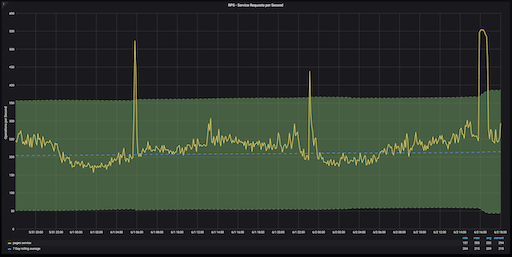
GitLab.com Pages service RPS over 48 hours, with ±3 z-score region in green
Z-scores are a bit awkward to interpret on a graph because they don’t have a unit of measurement. But anomalies on this chart are easy to detect. Anything that appears outside of the green area (which denotes z-scores that fall within a range of +3 or -3) is an anomaly.
What if you don’t have a normal distribution?
But wait: We make a big leap by assuming that our underlying aggregation has a normal distribution. If we calculate the z-score with data that isn’t normally distributed, our results will be incorrect.
There are numerous statistical techniques for testing your data for a normal distribution, but the best option is to test that your underlying data has a z-score of about +4 to -4.
(
 max_over_time(job:http_requests:rate5m[1w]) - avg_over_time(job:http_requests:rate5m[1w])
) / stddev_over_time(job:http_requests:rate5m[1w])
# --> {job="apiserver", environment="prod"}  4.01
# --> {job="gitserver", environment="prod"}  3.96
# --> {job="webserver", environment="prod"}  2.96

(
 min_over_time(job:http_requests:rate5m[1w]) - avg_over_time(job:http_requests:rate5m[1w])
) / stddev_over_time(job:http_requests:rate5m[1w])
# --> {job="apiserver", environment="prod"}  -3.8
# --> {job="gitserver", environment="prod"}  -4.1
# --> {job="webserver", environment="prod"}  -3.2
Two Prometheus queries testing the minimum and maximum z-scores.
If your results return with a range of +20 to -20, the tail is too long and your results will be skewed. Remember too that this needs to be run on an aggregated, not unaggregated series. Metrics that probably don’t have normal distributions include things like error rates, latencies, queue lengths etc., but many of these metrics will tend to work better with fixed thresholds for alerting anyway.
Detecting anomalies using seasonality
While calculating z-scores works well with normal distributions of time series data, there is a second method that can yield even more accurate anomaly detection results. Seasonality is a characteristic of a time series metric in which the metric experiences regular and predictable changes that recur every cycle.
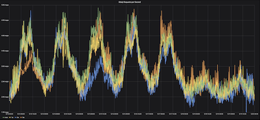
Gitaly requests per second (RPS), Monday-Sunday, over four consecutive weeks
This graph illustrates the RPS (requests per second) rates for Gitaly over seven days, Monday through Sunday, over four consecutive weeks. The seven-day range is referred to as the “offset,” meaning the pattern that will be measured.
Each week on the graph is in a different color. The seasonality in the data is indicated by the consistency in trends indicated on the graph – every Monday morning, we see the same rise in RPS rates, and on Friday evenings, we see the RPS rates drop off, week after week.
By leveraging the seasonality in our time series data we can create more accurate predictions which will lead to better anomaly detection.
How do we leverage seasonality?
Calculating seasonality with Prometheus required that we iterate on a few different statistical principles.
In the first iteration, we calculate by adding the growth trend we’ve seen over a one-week period to the value from the previous week. Calculate the growth trend by subtracting the rolling one-week average for last week from the rolling one-week average for now.
- record: job:http_requests:rate5m_prediction
  expr: >
    job:http_requests:rate5m offset 1w                     # Value from last period
    + job:http_requests:rate5m:avg_over_time_1w            # One-week growth trend
    - job:http_requests:rate5m:avg_over_time_1w offset 1w
The first iteration is a bit narrow; we’re using a five-minute window from this week and the previous week to derive our predictions.
In the second iteration, we expand our scope by taking the average of a four-hour period for the previous week and comparing it to the current week. So, if we’re trying to predict the value of a metric at 8am on a Monday morning, instead of using the same five-minute window from one week prior, we use the average value for the metric from 6am until 10am for the previous morning.
- record: job:http_requests:rate5m_prediction
  expr: >
    avg_over_time(job:http_requests:rate5m[4h] offset 166h) # Rounded value from last period
    + job:http_requests:rate5m:avg_over_time_1w             # Add 1w growth trend
    - job:http_requests:rate5m:avg_over_time_1w offset 1w
We use the 166 hours in the query instead of one week because we want to use a four-hour period based on the current time of day, so we need the offset to be two hours short of a full week.
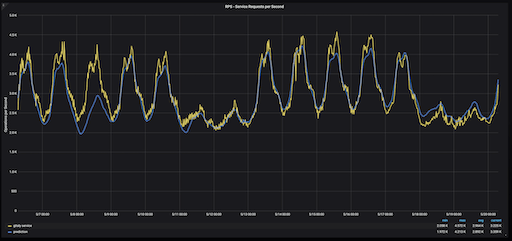
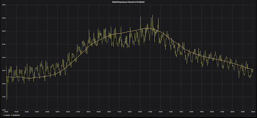
Gitaly service RPS (yellow) vs prediction (blue), over two weeks.
A comparison of the actual Gitaly RPS (yellow) with our prediction (blue) indicate that our calculations were fairly accurate. However, this method has a flaw.
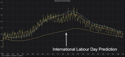
GitLab usage was lower than the typical Wednesday because May 1 was International Labor Day, a holiday celebrated in many different countries. Because our growth rate is informed by the previous week’s usage, our predictions for the next week, on Wednesday, May 8, were for a lower RPS than it would have been had it not been a holiday on Wednesday, May 1.
This can be fixed by making three predictions for three consecutive weeks before Wednesday, May 1; for the previous Wednesday, the Wednesday before that, and the Wednesday before that. The query stays the same, but the offset is adjusted.
- record: job:http_requests:rate5m_prediction
  expr: >
   quantile(0.5,
     label_replace(
       avg_over_time(job:http_requests:rate5m[4h] offset 166h)
       + job:http_requests:rate5m:avg_over_time_1w - job:http_requests:rate5m:avg_over_time_1w offset 1w
       , "offset", "1w", "", "")
     or
     label_replace(
       avg_over_time(job:http_requests:rate5m[4h] offset 334h)
       + job:http_requests:rate5m:avg_over_time_1w - job:http_requests:rate5m:avg_over_time_1w offset 2w
       , "offset", "2w", "", "")
     or
     label_replace(
       avg_over_time(job:http_requests:rate5m[4h] offset 502h)
       + job:http_requests:rate5m:avg_over_time_1w - job:http_requests:rate5m:avg_over_time_1w offset 3w
       , "offset", "3w", "", "")
   )
   without (offset)
Three predictions for three Wednesdays vs actual Gitaly RPS, Wednesday, May 8 (one week following International Labor Day)
On the graph we’ve plotted Wednesday, May 8 and three predictions for the three consecutive weeks before May 8. We can see that two of the predictions are good, but the May 1 prediction is still far off base.
Also, we don’t want three predictions, we want one prediction. Taking the average is not an option, because it will be diluted by our skewed May 1 RPS data. Instead, we want to calculate the median. Prometheus does not have a median query, but we can use a quantile aggregation in lieu of the median.
The one problem with this approach is that we're trying to include three series in an aggregation, and those three series are actually all the same series over three weeks. In other words, they all have the same labels, so connecting them is tricky. To avoid confusion, we create a label called offset and use the label-replace function to add an offset to each of the three weeks. Next, in the quantile aggregation, we strip that off, and that gives us the middle value out of the three.
- record: job:http_requests:rate5m_prediction
  expr: >
   quantile(0.5,
     label_replace(
       avg_over_time(job:http_requests:rate5m[4h] offset 166h)
       + job:http_requests:rate5m:avg_over_time_1w - job:http_requests:rate5m:avg_over_time_1w offset 1w
       , "offset", "1w", "", "")
     or
     label_replace(
       avg_over_time(job:http_requests:rate5m[4h] offset 334h)
       + job:http_requests:rate5m:avg_over_time_1w - job:http_requests:rate5m:avg_over_time_1w offset 2w
       , "offset", "2w", "", "")
     or
     label_replace(
       avg_over_time(job:http_requests:rate5m[4h] offset 502h)
       + job:http_requests:rate5m:avg_over_time_1w - job:http_requests:rate5m:avg_over_time_1w offset 3w
       , "offset", "3w", "", "")
   )
   without (offset)
Now, our prediction deriving the median value from the series of three aggregations is much more accurate.
Median predictions vs actual Gitaly RPS, Wednesday, May 8 (one week following International Labor Day)
How do we know our prediction is truly accurate?
To test the accuracy of our prediction, we can return to the z-score. We can use the z-score to measure the sample's distance from its prediction in standard deviations. The more standard deviations away from our prediction we are, the greater the likelihood is that a particular value is an outlier.
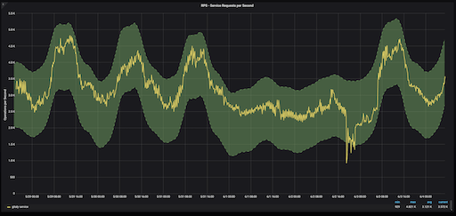
Predicted normal range ± 1.5σ for Gitaly Service
We can update our Grafana chart to use the seasonal prediction rather than the weekly rolling average value. The range of normality for a certain time of day is shaded in green. Anything that falls outside of the shaded green area is considered an outlier. In this case, the outlier was on Sunday afternoon when our cloud provider encountered some network issues.
Using boundaries of ±2σ on either side of our prediction is a pretty good measurement for determining an outlier with seasonal predictions.
How to set up alerting using Prometheus
If you want to set up alerts for anomaly events, you can apply a pretty straightforward rule to Prometheus that checks if the z-score of the metric is between a standard deviation of +2 or -2.
- alert: RequestRateOutsideNormalRange
  expr: >
   abs(
     (
       job:http_requests:rate5m - job:http_requests:rate5m_prediction
     ) / job:http_requests:rate5m:stddev_over_time_1w
   ) > 2
  for: 10m
  labels:
    severity: warning
  annotations:
    summary: Requests for job {{ $labels.job }} are outside of expected operating parameters
At GitLab, we use a custom routing rule that pings Slack when any anomalies are detected, but doesn’t page our on-call support staff.
The takeaway
- Prometheus can be used for some types of anomaly detection
- The right level of data aggregation is the key to anomaly detection
- Z-scoring is an effective method, if your data has a normal distribution
- Seasonal metrics can provide great results for anomaly detection
Watch Andrew’s full presentation from Monitorama 2019. If you have questions for Andrew, reach him on Slack at #talk-andrew-newdigate. You can also read more about why you need Prometheus.


